import SphericalSpatialTrees as SST
import GeometryOps as GO, GeoInterface as GI
import DiskArrays

using GeometryOps.UnitSpherical: GeographicFromUnitSphere, spherical_distance,
                            UnitSphereFromGeographic, SphericalCap

using Rasters, RasterDataSources, ArchGDAL, Zarr # data sources
using GeoMakie, GLMakie # visualization

"/home/runner/.julia/artifacts/RasterDataSources"

nothing # hide

Now that we have loaded all of these packages, let's start talking about functionality.

First, let's use the top-level interface to create a lazily regridded array, from a lat-long source to a DGGS target.

This dataset is a bioclimatic dataset, which is sufficiently small that you can do this quickly on your machine.

ras = Raster(EarthEnv{HabitatHeterogeneity}, :cv) |> r -> replace_missing(r, NaN) .|> log

┌ 1728×696 Raster{Float64, 2} ┐
├─────────────────────────────┴────────────────────────────────────────── dims ┐
  ↓ X Projected{Float64} -180.0:0.20833333333333334:179.79166666666669 ForwardOrdered Regular Intervals{Start},
  → Y Projected{Float64} 84.79166666666667:-0.20833333333333334:-60.0 ReverseOrdered Regular Intervals{Start}
├──────────────────────────────────────────────────────────────────── metadata ┤
  Metadata{Rasters.GDALsource} of Dict{String, Any} with 1 entry:
  "filepath" => "/home/runner/.julia/artifacts/RasterDataSources/EarthEnv/Habit…
├────────────────────────────────────────────────────────────────────── raster ┤
  missingval: NaN
  extent: Extent(X = (-180.0, 180.00000000000003), Y = (-60.0, 85.0))
  crs: GEOGCS["WGS 84",DATUM["WGS_1984",SPHEROID["WGS 84",6378137,298.25722...
└──────────────────────────────────────────────────────────────────────────────┘
    ↓ →     84.7917   84.5833   84.375  …  -59.375  -59.5833  -59.7917  -60.0
 -180.0    NaN       NaN       NaN         NaN      NaN       NaN       NaN
 -179.792  NaN       NaN       NaN         NaN      NaN       NaN       NaN
    ⋮                                   ⋱                       ⋮       
  179.583  NaN       NaN       NaN         NaN      NaN       NaN       NaN
  179.792  NaN       NaN       NaN         NaN      NaN       NaN       NaN

Let's give this dataset some chunks. It's 1728x696 so 75x75 chunks give it ~ 22x11 chunks.

ras_chunked = DiskArrays.mockchunks(ras, (75, 75))

┌ 1728×696 Raster{Float64, 2} ┐
├─────────────────────────────┴────────────────────────────────────────── dims ┐
  ↓ X Projected{Float64} -180.0:0.20833333333333334:179.79166666666669 ForwardOrdered Regular Intervals{Start},
  → Y Projected{Float64} 84.79166666666667:-0.20833333333333334:-60.0 ReverseOrdered Regular Intervals{Start}
├──────────────────────────────────────────────────────────────────── metadata ┤
  Metadata{Rasters.GDALsource} of Dict{String, Any} with 1 entry:
  "filepath" => "/home/runner/.julia/artifacts/RasterDataSources/EarthEnv/Habit…
├────────────────────────────────────────────────────────────────────── raster ┤
  missingval: NaN
  extent: Extent(X = (-180.0, 180.00000000000003), Y = (-60.0, 85.0))
  crs: GEOGCS["WGS 84",DATUM["WGS_1984",SPHEROID["WGS 84",6378137,298.25722...
└──────────────────────────────────────────────────────────────────────────────┘

Now, we need to define the source and target trees. The dataset itself is on a plane (equirectangular projection), so we can use the RegularGridTree which is an implicit quadtree.

source = SST.ProjectionSource(SST.RegularGridTree, ras_chunked);

We want to go to a DGGS target, so we can use the ISEACircleTree (based on the Snyder equal area projection). This is the only tree so far but more can be added as we go forward.

target = SST.ProjectionTarget(SST.ISEACircleTree, 8, 2)

ProjectionSource(655360-leaf ISEACircleTree(8))

As a sidenote, this is what actually happens internally. Using the spatial tree interface, we compute the map of chunks in the source dataset that each chunk in the target dataset requires to be materialized.

SST.compute_connected_chunks(source, target)

160-element Vector{Vector{Int64}}:
 [65, 66, 89, 90, 113, 114, 67, 91, 115, 92]
 [90, 114, 91, 115, 92, 116, 138, 139, 140]
 [115, 116, 138, 139, 140, 141, 163, 164]
 [139, 140, 141, 163, 164, 165, 188, 189]
 [41, 42, 65, 66, 89, 90, 43, 44, 67, 68, 91, 92]
 [66, 90, 67, 68, 69, 91, 115, 92, 93, 116]
 [91, 115, 92, 93, 116, 117, 139, 140, 141]
 [116, 117, 118, 140, 141, 164, 165, 142]
 [16, 17, 18, 40, 41, 42, 65, 66, 19, 20, 21, 43, 44, 45, 67, 68]
 [42, 66, 43, 44, 45, 46, 67, 68, 69, 91, 92, 93, 70]
 ⋮
 [209, 210, 233, 234, 211, 235, 212, 213, 236, 237]
 [112, 113, 114, 136, 137, 138, 160, 161, 162]
 [137, 138, 161, 162, 185, 186, 139, 163, 187]
 [161, 162, 185, 186, 209, 210, 163, 187, 188, 211]
 [186, 209, 210, 234, 187, 188, 189, 211, 235, 212, 213, 236, 237]
 [89, 90, 113, 114, 115, 137, 138, 139]
 [114, 115, 137, 138, 162, 139, 163]
 [138, 162, 186, 139, 140, 163, 164, 187, 188]
 [162, 186, 163, 164, 165, 187, 188, 189, 211, 212]

Now, we can create the lazy projected disk array.

a = SST.LazyProjectedDiskArray(source, target)

256×256×10 LazyProjectedDiskArray{Float64}

You can now access some data, using this as you would use any array:

a[1:10,1:10,1]

10×10 Matrix{Float64}:
 7.3815   7.04491  7.29845  7.52456  …  8.79301  8.80072  8.71997  8.69148
 7.54803  7.28893  7.00941  7.03791     9.16785  9.04958  8.76639  8.33399
 8.0523   7.43897  7.24494  6.9256      8.07465  8.97246  8.94637  8.41183
 7.40123  7.60589  7.6029   7.18007     7.4055   7.83241  8.55005  8.72013
 6.50728  7.98888  7.27656  7.04491     7.41035  8.18897  8.97094  8.71325
 6.86797  7.35756  8.0037   7.257    …  7.38956  7.64252  8.19008  8.97525
 7.02376  6.82871  7.13569  7.59085     7.13807  7.48212  7.71869  8.12976
 7.44425  6.92264  6.85013  6.58203     7.51698  7.57661  7.68064  7.85941
 7.44425  7.13966  7.0193   6.80793     7.59035  7.03351  7.29777  7.6019
 7.20564  7.50384  7.10168  7.11314     6.98008  7.49165  6.89264  7.02554

You can also materialize the array fully into memory (if the array is small enough):

ac = collect(a);

Now let's visualize this! GLMakie has no problem visualizing this many polygons: First, let's get every polygon:

polys = SST.index_to_polygon_lonlat.(vec(collect(eachindex(a))), (target.tree,));

Then we can just assign the correct color to the correct polygon, and plot on GeoMakie's GlobeAxis.

fig, ax, p1 = poly(a; axis = (; type = GlobeAxis))
p2 = lines!(ax, a; color = :black, transparency = true, linewidth = 0.075)
p3 = meshimage!(ax, -180..180, -90..90, fill(colorant"white", 2, 2); zlevel = -100_000)
fig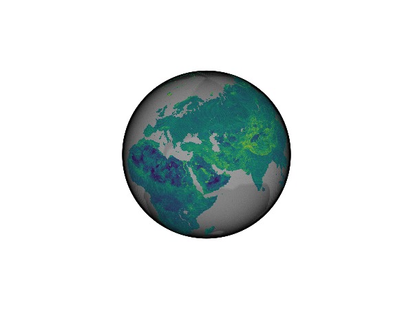

Let's also see the original data:

meshimage(-180..180, -90..90, reorder(ras, Y => Rasters.ForwardOrdered()); axis = (; type = GlobeAxis))

To give a better idea of what this looks like, let's use a lower level (lower resolution) DGGS:

target = SST.ProjectionTarget(SST.ISEACircleTree, 3, 2)
a = SST.LazyProjectedDiskArray(source, target)
ac = mapreduce((i,j)->cat(i,j,dims=3),1:10) do n
    a[:,:,n]
end
fig, ax, plt = poly(a; strokewidth = 1, strokecolor = :black, axis = (; type = GlobeAxis));
meshimage!(ax, -180..180, -90..90, fill(colorant"white", 2, 2); zlevel = -100_000) # background plot
fig

fig2, ax2, plt2 = meshimage(-180..180, -90..90, reorder(ras, Y => Rasters.ForwardOrdered()); zlevel = 100_000, alpha = 0.5, transparency = true, axis = (; type = GlobeAxis, show_axis = false))
poly!(ax2, a; strokewidth = 1, strokecolor = :black)
meshimage!(ax2, -180..180, -90..90, fill(colorant"white", 2, 2); zlevel = -100_000) # background plot

Makie.Plot{GeoMakie.meshimage, Tuple{Makie.EndPoints{Float64}, Makie.EndPoints{Float64}, Matrix{ColorTypes.RGB{FixedPointNumbers.N0f8}}}}

And that's the basics! Now we can go a bit into the weeds of capabilities and how this works.

mycoord = (11.0, 53.0)
rad = 1e-6

iseat = SST.ISEACircleTree(22)
mycircle = SphericalCap(UnitSphereFromGeographic()(mycoord), rad)

GeometryOps.UnitSpherical.SphericalCap{Float64}(UnitSphericalPoint(0.5907579861332358, 0.11483171997015439, 0.7986355100472928), 1.0e-6, 0.9999999999995)

Query

r = GO.query(iseat, mycircle)
points = SST.index_to_lonlat.(r, (iseat,))
f, a, p = scatter(points; color = Makie.Cycled(2), axis = (; type = GlobeAxis, show_axis = false));
lines!(a, GeoMakie.coastlines())
f

poly1 = SST.index_to_polygon_lonlat(1, iseat)

poly!(a, poly1; strokecolor = :red, strokewidth = 1)
f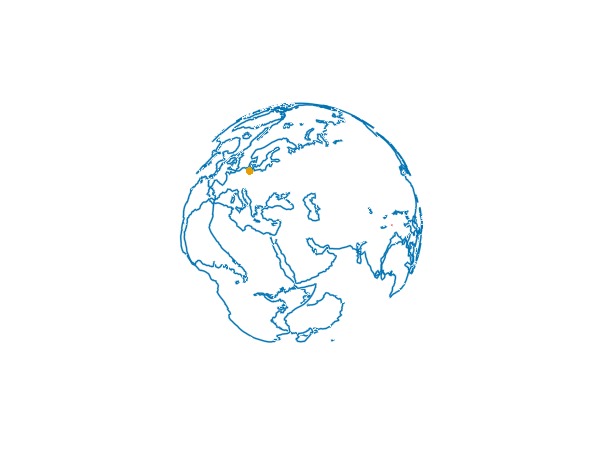

lo,up = CartesianIndices(SST.gridsize(iseat))[r] |> extrema
bb_isea = map(Colon(), lo.I, up.I)


ras = Raster(WorldClim{BioClim}, 5) |> r -> replace_missing(r, NaN)
c = DiskArrays.mockchunks(ras, DiskArrays.GridChunks(size(ras), (100, 100)))
lccst = SST.RegularGridTree(c)
r2 = GO.query(SST.rootnode(lccst), mycircle)
SST.index_to_lonlat.(r2, (lccst,))

lo, up = CartesianIndices(size(c)[1:2])[r2] |> extrema
bb_lccs = map(Colon(), lo.I, up.I)



d, i = SST.find_nearest(iseat, (11.0, 53.0))
SST.index_to_lonlat(i, iseat)

d, i = SST.find_nearest(lccst, (11.0, 53.0))
SST.index_to_lonlat(i, lccst)



source = SST.ProjectionSource(SST.RegularGridTree, c);
target = SST.ProjectionTarget(SST.ISEACircleTree, 3, 2);


SST.compute_connected_chunks(source, target)


a = SST.LazyProjectedDiskArray(source, target)

8×8×10 LazyProjectedDiskArray{Float64}

How do I get a polygon from a cartesian index?

SST.index_to_polygon_lonlat(CartesianIndex(1,1,1), target.tree)

GeoInterface.Wrappers.Polygon{false, false}([GeoInterface.Wrappers.LineString([(90.0, 26.56505117707799), … (3) … , (90.0, 26.56505117707799)], crs = "EPSG:4326")], crs = "EPSG:4326")

Let's get every polygon...

polys = SST.index_to_polygon_lonlat.(eachindex(a), (target.tree,));

This is

length(polys)

640

a[:, 1, :]

8×10 Matrix{Float64}:
  28.6612  NaN  NaN  NaN   37.7863  …  NaN        NaN       NaN
  30.2127  NaN  NaN  NaN   38.7557     NaN        NaN       NaN
  34.7407  NaN  NaN  NaN   41.8978     NaN        NaN       NaN
 NaN       NaN  NaN  NaN   27.984      NaN        NaN       NaN
  32.0272  NaN  NaN  NaN   36.2388     NaN        NaN       NaN
 NaN       NaN  NaN  NaN  NaN       …  NaN        NaN        -4.77825
 NaN       NaN  NaN  NaN   32.5433      -2.0865   -14.7845  -16.0435
  39.934   NaN  NaN  NaN  NaN           -9.90425  -19.6     -27.3525

Now we can materialize the lazy array...

@time ac = collect(a);

  0.089171 seconds (3.03 k allocations: 5.386 MiB)

and GLMakie has no problem visualizing this!

poly(vec(polys); color = vec(ac), strokewidth = 1, strokecolor = :black, axis = (; type = GlobeAxis, show_axis = false))
meshimage!(-180..180, -90..90, fill(colorant"white", 2, 2); zlevel = -100_000)
current_figure()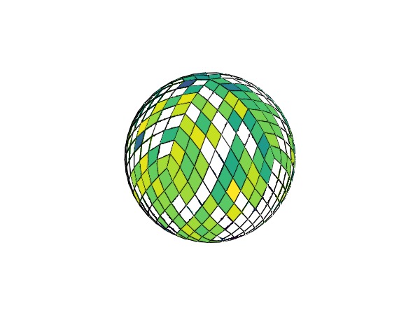

heatmap(c.lccs_class.data[bb_lccs...][:, :, 1])

ds = SST.create_dataset(target, "./output.zarr/", arrayname=:lccs_class)

SST.reproject!(ds.lccs_class,source,target)

---

This page was generated using Literate.jl.